
Databases
Why is my database query slow?
By Muhammad UmarJune 27, 202513 min readIssue #5
An index is an ordering, not a speed setting. Once you see that, most confusing database behaviour stops being confusing.
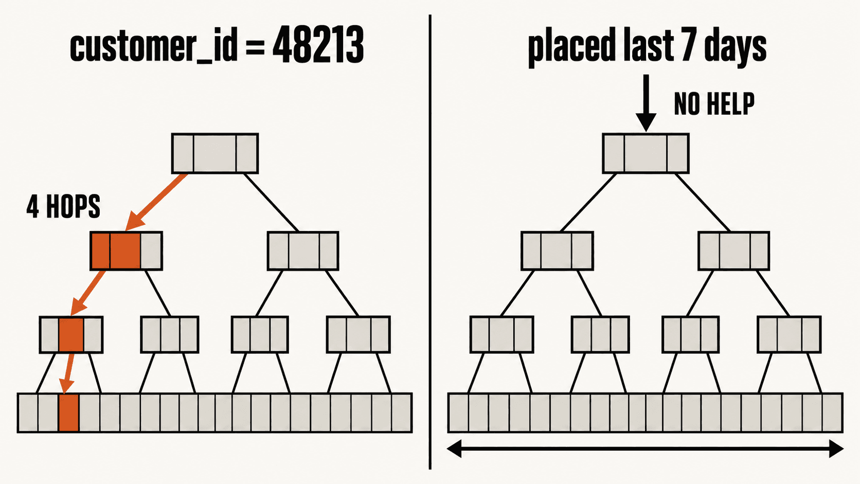
You've got a 900-page cookbook and you want every recipe that uses saffron. With no index, there's only one way to do it: open page one, read it, turn the page, read it, all the way to page 900. You'll find every saffron recipe. It'll just take you an afternoon.
The index at the back changes that. Flip to S, find saffron: 112, 340, 671, jump to three pages. Seconds instead of an afternoon.
Here's the part that matters, and it's the part most explanations skip. That index is fast because it's sorted alphabetically, and that same sorting is exactly why it can't help you find recipes that take under 30 minutes. The index doesn't know anything about time. It only knows letters.
That one sentence explains most of the confusing behaviour you'll ever see from a database index.
So let's start there, because “indexes make queries faster” is the belief that gets people stuck. It's not wrong exactly. It's just too vague to predict anything, and a model that can't predict anything is no use when your query is slow at two in the morning.
The problem, concretely
You have an orders table with ten million rows. This query used to be fine:
SELECT * FROM orders WHERE customer_id = 48213;Now it takes several seconds. So you do the reasonable thing and add an index:
CREATE INDEX idx_orders_customer ON orders (customer_id);The query gets fast. Excellent. Then you write this one:
SELECT * FROM orders
WHERE status = 'pending'
ORDER BY created_at DESC
LIMIT 50;
It's slow. You add an index on status. Still slow. You check whether the database is even using your new index, and it isn't. You've done everything you were told to do and the database is ignoring you.
Nothing has gone wrong. The database is behaving exactly as designed. You just need a better model of what an index is.
An index is an ordering, not a speed setting
Think about what makes the cookbook index useful. It isn't that it's smaller than the book, though it is. It's that it's sorted. Because the entries are in alphabetical order, you can skip enormous chunks of it without looking at them. You open to the middle, see M, and instantly know that saffron is in the second half. You never read the first half at all. Not quickly. Not at all.
That’s the whole trick. Sorting lets you eliminate most of the data without examining it.
A database index is the same idea. When you create an index on customer_id, the database builds a separate, sorted structure containing every customer_id value paired with a pointer to where that row physically lives. The table itself stays in whatever order it happened to be written. The index is the sorted copy.
And now the consequence, which is the useful bit: an index can only help with questions that its ordering can answer.
Sorted by customer ID? Then “find customer 48213” is easy, and so is “find customers between 48000 and 49000”, because sorted order means those sit next to each other. But “find orders placed in the last week” gets no help at all from that index, in the same way the alphabetical cookbook index gives you nothing when you ask about cooking time.
Once you hold that idea, the confusing cases stop being confusing. Every one of them is the same question: does the ordering I built actually answer the question I am asking?
What's actually in there
The structure almost every database reaches for by default is a B-tree. PostgreSQL uses one for CREATE INDEX unless you ask for something else, and its implementation follows the Lehman–Yao design, which is a variant built to let many readers and writers work on the tree at once without blocking each other.1
Picture it as a small stack of signposts sitting above your sorted data.
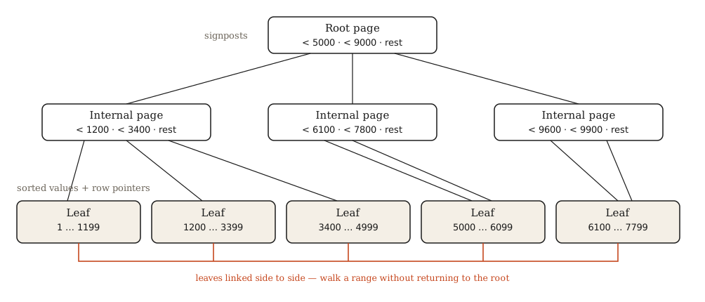
The bottom row, the leaves, holds the actual indexed values in sorted order, each with a pointer to the row in the table. Everything above is signposts: values below 5000 go left, below 9000 go middle, otherwise right. To find a value you start at the top and follow signposts down. Three or four hops and you are there.
Two details make this fast, and both are worth understanding rather than memorising.
The tree is extremely shallow
PostgreSQL reads and writes in fixed-size pages, 8 KB by default.2 A single 8 KB page holds a few hundred index entries, so each signpost page can point to a few hundred children. That branching factor compounds viciously: three levels reach on the order of hundreds of millions of entries, four levels reach far beyond anything you are likely to store. The practical consequence is that looking up a value costs roughly four page reads whether your table has one million rows or one hundred million. Growth barely touches it.
Compare that with the sequential scan, which reads every page of the table. Ten million rows might be hundreds of thousands of pages. Four reads against several hundred thousand is the entire difference, and it is why the first query got fast.
The leaves are linked side to side
Once you have found the start of a range you can walk sideways through the leaves without going back up through the tree. That is what makes BETWEEN, >, <, and ORDER BY on an indexed column cheap, and it is precisely the cookbook behaviour of reading straight down the S column once you have found it.
Four kinds of index, and when each is wrong
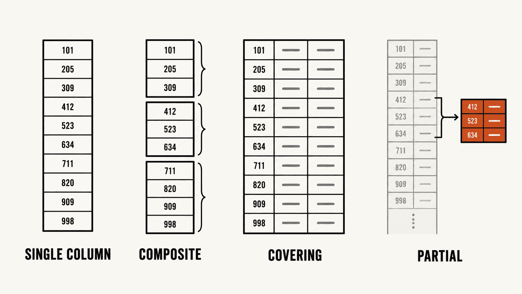
Single-column
One column, sorted. The default, and usually correct.
Wrong when your queries filter on two columns together. Two separate single-column indexes are not equivalent to one index covering both. PostgreSQL can combine them by building bitmaps of matching rows and intersecting those. That is a real capability, but the documentation is direct that a multicolumn index is generally better for a filter you run often, because the bitmap approach has to process both indexes in full.3
Composite
One index over several columns, sorted by the first, then by the second within each first value, and so on.
CREATE INDEX idx_orders_status_created
  ON orders (status, created_at);
This is the cookbook sorted first by ingredient, then by cooking time within each ingredient. Ask for saffron recipes, quickest first and it is laid out ready for you.
Column order is not cosmetic. That index serves WHERE status = 'pending', and it serves the same filter with ORDER BY created_at. It is far less useful for a filter on created_at alone, because those values are scattered, sorted only within each status group, not globally. PostgreSQL can still use the index for a non-leading column, but only by scanning the whole thing, which is often no better than scanning the table.3
The rule that follows: the leftmost columns are the ones that do the work. Put the column you filter on exact equality first, and the column you sort by or scan a range on after it.
Wrong when you are tempted to add a fourth and fifth column just in case. Every extra column widens each index entry, so fewer entries fit per 8 KB page, so the tree grows, and every insert has to write all of it. You pay that on each write, in exchange for serving fewer queries than you imagine.
Covering
An index that carries enough data to answer the query without touching the table at all. PostgreSQL supports an INCLUDE clause for payload columns that aren't part of the sort order.4
CREATE INDEX idx_orders_customer_covering
  ON orders (customer_id) INCLUDE (total_amount);
Now a query selecting only total_amount for one customer can be satisfied from the index alone: an index-only scan.
There's a catch that surprises people, and it's a good example of why reading the source beats reading the tutorial. PostgreSQL's index entries don't record whether a row version is visible to your transaction, so an index-only scan still has to confirm visibility. It does this through the visibility map, a compact structure marking which table pages are known all-visible. If the relevant page isn't marked, the scan falls back to reading the table row anyway.5 The visibility map is maintained by VACUUM, which is why an index-only scan can quietly stop being index-only on a heavily updated table that hasn't been vacuumed recently.
Wrong when the included columns are wide or updated frequently. You are duplicating data into the index and paying to maintain both copies.
Partial
An index over a subset of rows.
CREATE INDEX idx_orders_pending
  ON orders (created_at)
  WHERE status = 'pending';
If 2% of your orders are pending, this index is roughly 2% of the size of the equivalent full index. Small indexes stay cached in memory, and cached beats uncached by a margin that dwarfs most other optimisations.
Wrong when the predicate doesn't match your queries closely. PostgreSQL will only use a partial index when it can prove the query's WHERE clause implies the index's, and that proof engine is deliberately limited, so a condition that's obviously equivalent to you may not be provable to it.6
| Type | Best for | Main cost | Fails when |
|---|---|---|---|
| Single-column | One filter column | One index to maintain | Multi-column filters |
| Composite | Filter and sort together | Larger; column order matters | Query does not start at the leading column |
| Covering | Read-heavy, few columns | Duplicated data | Table is not vacuumed; wide columns |
| Partial | Skewed data, hot subset | Fragile matching rules | Predicate does not match the query |
What every index costs you
Selectivity, or why your status index was ignored
Back to the query that stayed slow. Here's the thing that explains it.
Suppose status = 'pending' matches 40% of your ten million rows. Using the index means: walk the index to collect four million row pointers, then fetch four million rows from the table, and those rows are scattered all over the disk, in whatever order they were written. Four million scattered lookups.
Or the database can read the table straight through, in physical order, and throw away the 60% that don't match.
Reading straight through wins, and it isn't close. PostgreSQL prices this explicitly: seq_page_cost defaults to 1.0 and random_page_cost to 4.0, encoding the assumption that a scattered page read costs about four times a sequential one.7 The planner adds up those costs and picks the cheaper plan. It didn't ignore your index out of stubbornness. It priced both options and your index lost.
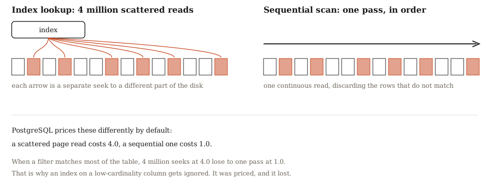
The general rule: an index earns its keep when it eliminates most of the table. A column with two values eliminates roughly half, which is nowhere near enough. A customer_id column with a million distinct values eliminates essentially everything, which is why the first query got fast and the second did not.
This is also the honest answer to “should I index this boolean?” Usually no. Unless the distribution is heavily skewed and you only ever query the rare side, in which case a partial index on that side is the right shape.
Every index taxes every write
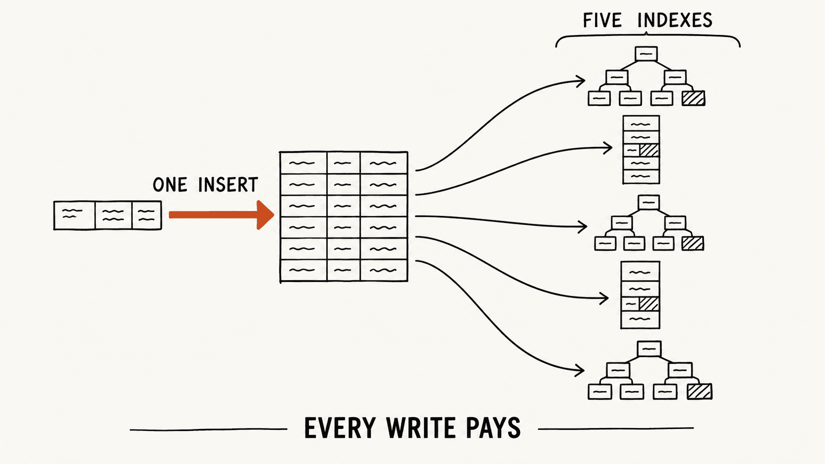
An index is a second copy of your data that has to stay correct. Insert a row and every index on that table must be updated. Same for deletes. This is the cost that doesn't show up in your query timings. It shows up as write throughput you never had.
PostgreSQL has a genuinely clever mitigation called HOT, heap-only tuple updates. When an update doesn't change any indexed column and the new row version fits on the same page as the old one, PostgreSQL can link the versions within the page and skip updating the indexes entirely.8 Both conditions have to hold. Update an indexed column, or fill the page, and you are back to paying full price on every index.
The practical read: indexes on columns you update constantly are expensive twice over: once for the index maintenance, once for the HOT optimisation you lose.
The planner is estimating, and estimates can be wrong
The cost model runs on statistics gathered by ANALYZE: row counts, value distributions, most common values. When those statistics are stale or the data is skewed in a way the sample missed, the planner makes a well-reasoned decision from bad numbers.
Read the plan, do not guess
EXPLAIN ANALYZE runs the query and reports both what the planner expected and what actually happened.9
EXPLAIN ANALYZE
SELECT * FROM orders
WHERE status = 'pending'
ORDER BY created_at DESC
LIMIT 50;
You get a tree of nodes. Three things are worth your attention before anything else.
Estimated versus actual rows. Every node reports rows= (the estimate) and actual rows= (the truth). When those differ by an order of magnitude or more, the planner was working from bad information, and every decision downstream of that node is suspect. The fix is usually ANALYZE, or raising the statistics target on a skewed column, not adding another index.
Which scan you got. Seq Scan reads the whole table. Index Scan walks the index and fetches rows one at a time. Bitmap Heap Scan sits in between: it collects matching locations from the index first, sorts them into physical order, then reads the table in one pass. That is the planner’s answer to “this index matches too many rows to fetch individually, but not so many that I should read everything”.10 Seeing a bitmap scan is not a problem. It is often the correct choice.
Where the time actually went. Times accumulate up the tree, so a node's own cost is its total minus its children's. A node reporting 900 ms whose children account for 880 ms is not your problem, however alarming the number looks.
The workflow that follows is unglamorous and reliable: measure, find the node where estimates diverge from reality or where the time genuinely goes, fix that one thing, measure again. Adding indexes speculatively is how tables end up carrying fifteen of them, of which four are ever used and all fifteen slow down every write.
Your database might not use B-trees at all
Everything above assumes a B-tree, and for PostgreSQL, MySQL's InnoDB, and most relational databases you'll meet, that's right.
But B-trees make a specific bet: updates happen in place. Change a value and the database finds the right page and rewrites it. That is excellent for reads and increasingly awkward for write-heavy workloads, because random in-place writes are the thing storage hardware likes least.
Log-structured merge trees take the opposite bet. Writes go to an in-memory table and a sequential log, and get merged down into sorted files on disk in the background. Writes become sequential and fast. Reads get harder, because a key might live in any of several files, so lookups check a chain of them. Bloom filters reduce that, but the cost is real.11 This is the design behind RocksDB, and behind Cassandra and ScyllaDB.
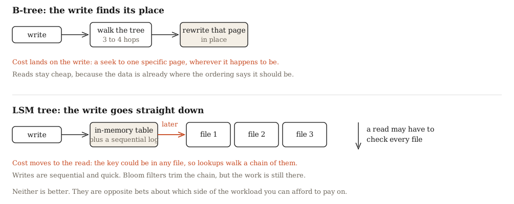
B-trees optimise reads and pay on writes. LSM trees optimise writes and pay on reads.
Neither is better. They are answers to different questions, and knowing which bet your storage engine made tells you which way its performance will bend under load.
Then there are the shapes B-trees genuinely can't handle, each with its own structure. Full-text search needs an inverted index: GIN, in PostgreSQL. Geospatial queries need something that can order two dimensions at once: GiST and SP-GiST. Vector similarity search needs approximate nearest-neighbour structures like HNSW, because exact nearest-neighbour in high dimensions degrades toward scanning everything.
All of them are the same idea the cookbook started with, applied to a different question: build an ordering that matches how you are going to ask.
That is the whole discipline. Not “add indexes to make things fast”. Decide what question you are asking, then build the ordering that answers it.
Sources
- PostgreSQL source,
src/backend/access/nbtree/README. The Lehman–Yao high-concurrency B-tree variant and PostgreSQL’s modifications to it. - PostgreSQL documentation, Database Page Layout. Default block size is 8192 bytes.
- PostgreSQL documentation, Multicolumn Indexes and Combining Multiple Indexes.
- PostgreSQL documentation, CREATE INDEX. The
INCLUDEclause, added in PostgreSQL 11. - PostgreSQL documentation, Index-Only Scans and Covering Indexes. Visibility map dependency and fallback to heap access.
- PostgreSQL documentation, Partial Indexes. Includes the limits of the predicate-implication proof.
- PostgreSQL documentation, Planner Cost Constants.
seq_page_costdefault 1.0,random_page_costdefault 4.0. - PostgreSQL source,
src/backend/access/heap/README.HOT. Conditions under which heap-only tuple updates avoid index maintenance. - PostgreSQL documentation, Using EXPLAIN.
- PostgreSQL documentation, Combining Multiple Indexes. Bitmap scans and the ordering of heap access.
- O’Neil, Cheng, Gawlick and O’Neil, The Log-Structured Merge-Tree (LSM-Tree), Acta Informatica 33, 1996.